26  Midterm Review

Author

Affiliation

Dr Randy Johnson

Hood College

Acknowledgements

These notes are an AI summary of the weekly lecture notes, with some light editing.

Week 1: Intro to Bioinformatics

What is Bioinformatics?

Bioinformatics is an interdisciplinary field that combines biology, computer science, and statistics. It focuses on the computational and statistical analysis of biological data to extract meaningful insights. This includes developing the software and methods used for these analyses.

Why is Bioinformatics Important?

The field is experiencing rapid growth due to the exponential increase in biological data and available computing power. It is crucial because it:

• Supports the transition of biology into a data-driven science.

• Is essential for processing, analyzing, and interpreting massive datasets, such as genetic information and protein structures.

• Helps organize, store, and retrieve diverse biological data.

• Facilitates a deeper understanding of cellular mechanisms and disease.

The Central Dogma & Molecular Basics

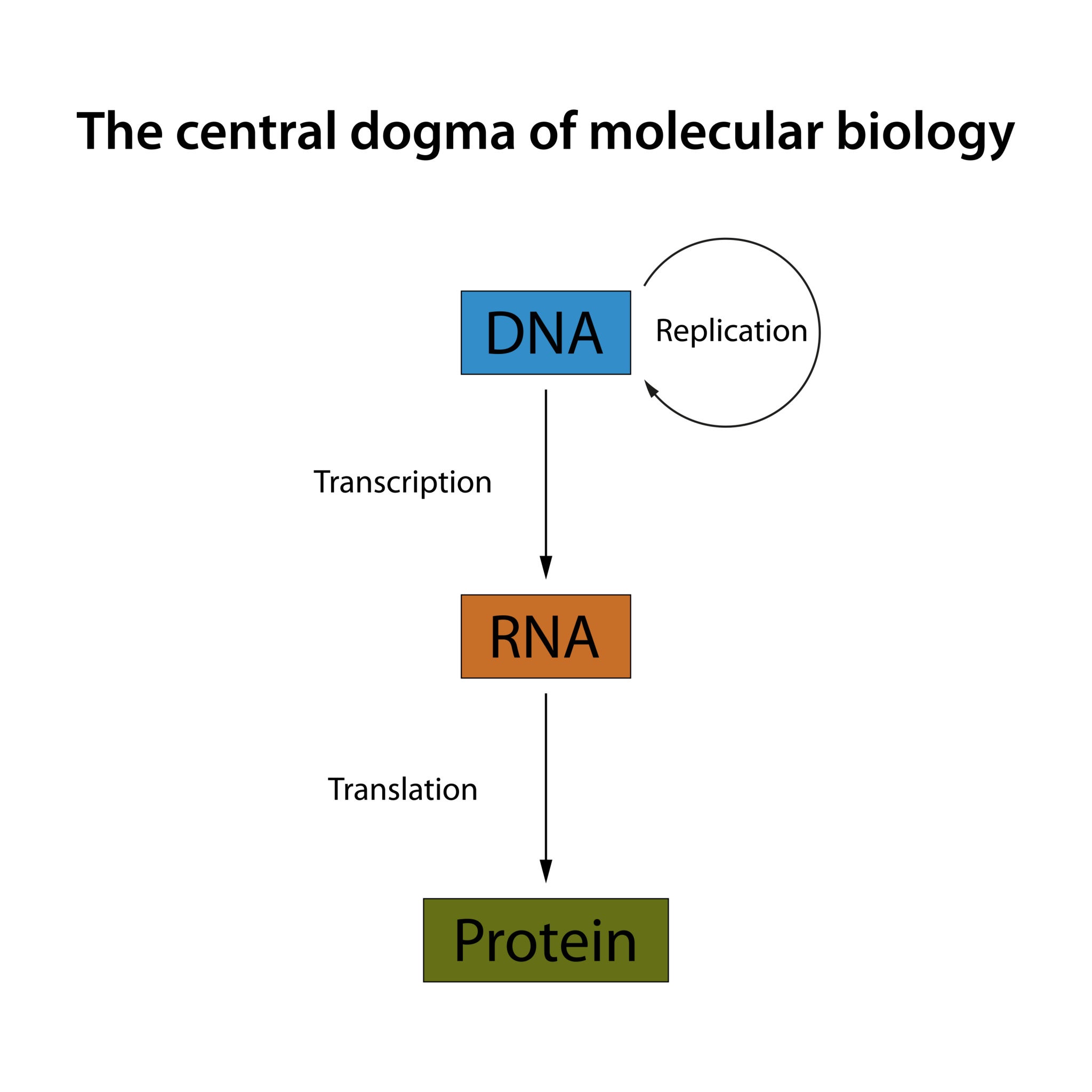
The original concept of the Central Dogma of Molecular Biology states that genetic information flows in one direction:

1. DNA transcription to RNA

2. RNA translation to protein

Some exceptions exist, such as RNA viruses (e.g., HIV, COVID-19) and prions, which are infectious proteins.

All DNA is composed of four nucleotides: Adenine (A), Guanine (G), Thymine (T), and Cytosine (C).

• Transcription: During this process, RNA polymerase binds to a DNA strand at a promoter and creates an RNA copy.

• Translation: The transcribed mRNA enters the cytoplasm and is read by a ribosome, one codon (a triplet of nucleotides) at a time, to build a protein. Thymine is transcribed to Uracil (U) in mRNA.

Key Tasks in Bioinformatics

• Genome Annotation: The process of identifying and labeling key features within a genome. This often begins by identifying Open Reading Frames (ORFs), which are DNA sequences that can be translated into proteins.

• Functional Annotation: This step assigns a biological function to predicted genes, often using Gene Ontology (GO) terms across three categories: Molecular Function, Biological Processes, and Cellular Components.

Biological Databases

Due to the sheer size of biological data, specialized databases are necessary for storage, management, and retrieval. These databases should follow the FAIR principles (Findable, Accessible, Interoperable, Reusable).

• Primary Databases: Contain raw, experimental data. Examples include GenBank (the most widely used database for DNA sequences), the European Nucleotide Archive (ENA), and the Sequence Read Archive (SRA).

• Secondary Databases: Contain curated and interpreted data derived from primary databases. Examples include UniProt (a major protein database), the Protein Data Bank (PDB) for 3D protein structures, and KEGG for pathway maps.

Common Tools and Applications

• FASTA Format: A simple text-based format for representing nucleotide or amino acid sequences.

• BLAST: The most frequently used tool for comparing a query sequence against a database to find regions of similarity.

• Key Application Areas:

  • Protein ID: Identifying and quantifying proteins from mass spectrometry data (e.g., MASCOT, MaxQuant).

  • Protein Structure Prediction: Predicting a protein’s 3D shape from its amino acid sequence (e.g., AlphaFold).

  • Drug Discovery: Using computational methods for virtual screening and ligand docking.

  • Gene Expression Analysis: Analyzing data from techniques like RNA-Seq.

  • Reconstructing Biological Networks: Visualizing complex protein interactions (e.g., using Cytoscape).

Future Directions

The field is moving toward integrating AI/Machine Learning and combining different data types (multi-omics data integration) to tackle more complex biological questions.

Week 2: Sequence Alignment & Search

Review of Key Concepts

Bioinformatics is an interdisciplinary field at the intersection of biology, mathematics, statistics, and computer science. The central dogma of molecular biology states that genetic information flows from DNA -> RNA -> Protein. Important bioinformatics databases include NCBI, UniProt, Protein Data Bank, and KEGG.

Sequence Alignment Concepts

What is Sequence Alignment?

Sequence alignment is the comparison of two or more biological sequences (DNA, RNA, or protein) to identify regions of similarity. These similarities can indicate functional, structural, or evolutionary relationships. Alignments account for matches, mismatches, and gaps (insertions or deletions, or indels).

Why is it Important?

• Identify homology and evolutionary relationships: This is the primary use. Two sequences are homologous if they share a common ancestor.

• Predict protein function and structure: Aligning a new sequence to a known homolog can help infer its potential function or structure.

• Design experiments: Conserved regions identified through alignment are critical for tasks like designing primers for PCR.

Key Terminology

• Homology: A fundamental similarity based on common descent.

• Orthologs: Homologous genes in different species that diverged after a speciation event (e.g., human and mouse hemoglobin genes).

• Paralogs: Homologous genes that diverged after a gene duplication event within the same species.

• Scoring Matrices: Tables that assign scores to matches and mismatches. Common examples include BLOSUM and PAM.

• Gap Penalties: Scores subtracted from the alignment score for introducing or extending a gap.

Pairwise Sequence Alignment

This method compares two sequences to determine their degree of similarity.

• Dynamic Programming Algorithms: These methods are computationally intensive but guarantee an optimal alignment.

  • Needleman-Wunsch Algorithm: Used for global alignments, aligning sequences across their entire length.

  • Smith-Waterman Algorithm: Used for local alignments, identifying the most similar regions within two sequences.

• Heuristic Algorithms: Provide a very good approximation quickly, making them practical for large datasets. BLAST is a prime example of a heuristic algorithm.

Searching Databases with BLAST

The Basic Local Alignment Search Tool (BLAST) is a widely used program for rapidly comparing a query sequence against a large database. It is a heuristic algorithm that finds regions of local similarity.

• How it Works: It uses a k-tuple/word method to quickly find matches, then extends these matches to create High-Scoring Pairs (HSPs).

• Key Implementations:

  • BLASTn: Nucleotide query vs. nucleotide database.

  • BLASTp: Protein query vs. protein database.

  • BLASTx: Translated nucleotide query vs. protein database.

  • tBLASTn: Protein query vs. translated nucleotide database.

• Interpreting Results: The E-value is a crucial statistical measure; a smaller E-value indicates a more significant match.

Multiple Sequence Alignment (MSA)

MSA is the simultaneous alignment of three or more sequences.

• Applications:

  • Identify conserved regions: Reveals functionally important patterns.

  • Infer evolutionary relationships: A prerequisite for constructing phylogenetic trees.

• Common Tools: Most MSA tools use a progressive alignment strategy, including ClustalOmega, MUSCLE, and MAFFT.

• Reciprocal Best Hits (RBH): A common strategy to identify orthologs and filter out paralogs. If gene A in species 1 is the best BLAST hit for gene B in species 2, and vice versa, they are likely orthologs.

Week 3: Next-Generation Sequencing

Introduction to Next-Generation Sequencing (NGS)

Next-Generation Sequencing (NGS), also known as massive parallel sequencing, is a technology that allows for the rapid, high-throughput, and cost-effective sequencing of DNA and RNA. It represents a major shift from the slower and more expensive Sanger sequencing method, which was based on the chain terminator method using dideoxynucleotides (ddNTPs). NGS technology enabled the sequencing of small DNA fragments in parallel, which greatly reduced costs and time.

NGS Platforms

NGS platforms fall into two main categories based on read length.

Short-Read Technologies (Second-Generation)

• Illumina: This is the most widely used platform today. It sequences DNA fragments attached to a flow cell by adding fluorescently labeled nucleotides in cycles. The emitted fluorescence is imaged to identify the incorporated base, and this process is repeated to build the sequence. Illumina produces short reads (50-250 bp) with high accuracy.

• Ion Torrent: This benchtop sequencer uses an ion semiconductor chip to detect hydrogen ions (H+) released during DNA polymerization. It is known for its portability, speed, and ease of use, making it ideal for clinical and infectious disease research.

Long-Read Technologies (Third-Generation)

These technologies directly sequence native DNA without prior fragmentation and amplification. They produce significantly longer reads, which are valuable for assembling complex genomes with repetitive regions.

• Pacific Biosciences (PacBio): PacBio’s single-molecule, real-time (SMRT) sequencing immobilizes a single DNA polymerase in a tiny well. Fluorescently labeled nucleotides are added and a light pulse is detected as each is incorporated. PacBio produces very long reads (>15 Kb) but with higher error rates, particularly for indels.

• Oxford Nanopore Technologies (ONT): The portable MinIon device sequences DNA by passing a single-stranded molecule through a nanopore. As the DNA passes through, it causes distinct changes in the ionic current, which are characteristic of the specific nucleotide bases. ONT produces variable and very long reads (sometimes up to 900 Kb), offering real-time data analysis.

NGS Data and Quality Assessment

The raw data from an NGS run consists of millions of reads, typically stored in a FASTQ file. This format includes both the nucleotide sequence and a corresponding Phred score for each base, which is a logarithmic measure of the probability of an incorrect base call (Q=−10log10​(p)). Higher Phred scores indicate greater confidence in the base call.

Initial quality control (QC) is a critical first step using tools like FastQC to assess base call quality and identify potential issues.

NGS Data Analysis Workflow

The primary goal of bioinformatics in NGS is to extract biological meaning from the raw data.

1. Preprocessing: This stage involves several steps to clean the raw data.

   • Demultiplexing: Separating pooled samples that were sequenced together using unique DNA barcodes.

   • Trimming and Filtering: Removing low-quality bases, adapter sequences, and short or low-quality reads.

   • Denoising: Correcting errors introduced during sequencing.

2. Sequence Assembly: The goal is to reconstruct longer, contiguous DNA sequences (contigs or scaffolds) from the short reads.

   • De novo assembly: Used when no reference genome is available.

   • Reference-guided assembly: Aligning reads to an existing, closely related reference genome.

3. Annotation: The process of identifying and labeling all relevant biological features within the assembled sequence, such as coding genes and other structural genes.

4. Quantification & Differential Expression Analysis: In a transcriptomics (RNA-seq) experiment, reads are aligned to a reference genome and counted to determine gene expression levels. Differential gene expression (DGE) analysis statistically identifies genes whose expression levels change significantly between experimental conditions.

5. Downstream Interpretation: This final stage involves various types of analysis and visualization to interpret the results.

   • Visualization: Tools like Volcano plots and MA-plots are used to visualize differential expression data. Principal Component Analysis (PCA) and Uniform Manifold Approximation and Projection (UMAP) are used for dimensionality reduction to visualize data clustering.

   • Enrichment Analysis: Identifies biological pathways that are statistically over-represented in a list of differentially expressed genes.

   • Machine Learning: Increasingly used for tasks like sample clustering, classification, and protein structure prediction (AlphaFold).

Challenges

NGS data science presents challenges related to the massive data volume and the required computational resources. Other issues include data quality problems like sparsity, missing values, and noise.

I hope this helps you prepare for your class. Let me know if you would like me to elaborate on any of the sections, such as the different sequencing chemistries or the specific data analysis tools.

Week 4: NGS Assembly & Annotation

Making Sense of NGS Data

Raw sequencing reads are fragmented pieces of DNA that are meaningless on their own. The goal of bioinformatics is to piece them together and interpret them to extract useful biological information. This process involves two primary steps: Genome Assembly and Genome Annotation.

Initial data processing steps include Base Calling, which converts raw signals into nucleotides and quality scores, and Trimming and Quality Control (QC), which removes low-quality data to reduce noise.

Genome Assembly

Genome assembly is the process of reconstructing a complete genome from millions of short sequencing reads. There are two main approaches:

• De Novo Assembly: This approach reconstructs a genome from scratch without using a pre-existing reference. It is used for new organisms or to find large-scale structural variations.

  • Algorithms:

    • Overlap-Layout-Consensus (OLC): Historically used for Sanger reads, this method is computationally intensive.

    • De Bruijn Graphs: More efficient for short-read data, this method breaks reads into small, overlapping “k-mers” that become nodes in a graph.

  • Tools: SPAdes, Velvet, and Flye are common tools.

• Reference-Guided/Assisted Assembly: This approach aligns sequencing reads to a known, closely related reference genome. It is faster and less computationally demanding but may introduce biases.

  • Tools: BWA, Bowtie, and HISAT2 are widely used for this purpose.

Challenges in Assembly include resolving repetitive sequences, dealing with high heterozygosity, and handling gaps where no reads could be assembled. Long-read technologies like PacBio and Nanopore are often preferred for generating a fully closed genome.

Genome Annotation

Genome annotation is the process of identifying and labeling all biologically meaningful features within an assembled DNA sequence. This includes:

• Identifying Noncoding Regions: Labeling repetitive elements, transposable elements, and noncoding RNAs (e.g., tRNAs, rRNAs).

• Gene Prediction: Identifying potential protein-coding genes, typically by finding Open Reading Frames (ORFs), which are stretches of DNA that can be translated without a stop codon.

Approaches to Annotation:

• Ab Initio Prediction: Uses computational models to predict genes based on their characteristics without external evidence.

• Evidence-Based Prediction: Aligns experimental data, such as RNA-seq data, to the genome to support gene predictions.

• Functional Annotation: Assigns a biological function to the identified features using methods like Homology Search (e.g., BLAST) against databases like UniProt and by mapping Gene Ontology (GO) Terms using tools like BlastKOALA.

Annotation Tools:

• Automatic Pipelines: Offered by NCBI and Ensembl, these are fast and flexible.

• Specialized Servers: RAST is commonly used for prokaryotic genomes, while BlastKOALA and GhostKOALA are used for functional annotation.

• Software Suites: Prokka is a popular tool for rapid prokaryotic genome annotation.

Challenges in Annotation include the trade-off between the speed of automatic pipelines and the accuracy of time-consuming manual curation. Additionally, annotations can become outdated, and it is more difficult to annotate genomes from non-model organisms.

Future Perspectives

The field is continuously advancing, with Deep Learning playing an increasingly important role. Deep learning models are being applied to improve the accuracy of genome annotation and functional prediction with tools like DeepAnnotator, DeepGOPlus, and AlphaGenome.

Weeks 5 & 7: Bulk RNA-seq

What is Transcriptomics?

Transcriptomics is the study of the entire set of RNA transcripts (the transcriptome) present in a cell or organism at a specific time or under specific conditions. It is based on the central dogma of molecular biology, which states that genetic information flows from DNA to RNA to protein. By measuring the amount of messenger RNA (mRNA) transcribed, we can estimate how active a gene is, providing insights into gene regulation and an organism’s phenotype.

Licensed by Google

Evolution of Gene Expression Analysis Technologies

• Northern Blotting: An early method for detecting the presence of specific RNA sequences. It was limited because it could only analyze one or a few targets at a time.

• Quantitative PCR (qPCR): An improvement that allowed for the faster quantification of several RNA targets simultaneously. It still relied on knowing what you were looking for and using specific probes.

• Microarrays: These enabled the simultaneous quantification of thousands of RNA targets from two different samples. Microarrays provided a broader view than previous methods but were still limited to the probes on the chip.

These traditional methods were all limited because they relied on specific probes and primers, meaning you could only find what you were looking for.

RNA Sequencing (RNA-Seq)

As the cost of NGS decreased, RNA-Seq replaced traditional hybridization techniques for genome-wide expression studies. RNA-Seq uses high-throughput sequencing to provide a much broader and unbiased view of the transcriptome.

Applications of RNA-Seq include:

• Differential Gene Expression (DGE) analysis

• Transcript discovery (e.g., non-coding RNAs)

• Differential alternative splicing

• Genome annotation

Key Experimental Design Considerations:

• Biological Replicates: At least three biological replicates are needed to increase statistical power and account for random variation.

• Sequencing Platform: Illumina short-read technology is common, but long-read technologies can be used for alternative splicing. Single-cell RNA-seq (scRNA-seq) uses platforms like 10x Genomics.

• Sequencing Strategy: Paired-end sequencing improves mapping accuracy, while single-end is less expensive.

• Sequencing Depth: Higher depth ensures better detection of lowly expressed genes.

RNA-Seq Data Analysis Workflow

1. Library Preparation: RNA is extracted, depleted of rRNA, fragmented, and converted to complementary DNA (cDNA). Sequencing adapters and barcodes are then added to the fragments for multiplexing.

2. Quality Control (QC): Raw data is checked using tools like FastQC, and low-quality bases, adapter sequences, and short reads are removed using Trimmomatic.

3. Mapping and Processing: Reads are aligned to a reference genome using tools like STAR Aligner. The output is then processed (sorted and indexed) using tools like Samtools.

4. Expression Quantification: The number of reads mapping to each gene is counted using tools like Subread to create a count matrix.

5. Normalization: This is a crucial step to account for biases in sequencing depth and data composition. Common methods include RPKM and FPKM.

6. Differential Gene Expression (DGE) Analysis: Statistical analysis using tools like DESeq2 and EdgeR is performed to identify genes whose expression levels change significantly between different conditions. It is essential to account for multiple hypothesis testing using methods like Benjamini–Hochberg to reduce false positives.

7. Downstream Analysis:

   • Visualization: Volcano plots and MA-plots visualize differential expression. Principal Component Analysis (PCA) and UMAP are used for dimensionality reduction to visualize data clustering.

   • Enrichment and Pathway Analysis: Identifies biological pathways and gene sets that are over-represented in the results. Tools like GO terms and KEGG are used for this.

RNA-Seq Data Analysis Workflow: A Closer Look

Here is a more detailed look at the key steps in a typical RNA-seq analysis pipeline, often using tools from the Bioconductor project in R.

Data Wrangling

The first step is to import the data into an analysis environment. This involves reading the raw gene count matrix (genes x samples) and adding sample metadata, such as experimental groups and batches. Tools like edgeR::readDGE are commonly used for this.

Data Pre-processing

• Filtering: Genes with consistently low expression across all samples are removed. This focuses the analysis on genes with sufficient statistical power and reduces the multiple testing burden.

• Normalization: Data is normalized to account for differences in sequencing depth (library size) and compositional biases. The Trimmed Mean of M-values (TMM) method, calculated by edgeR::calcNormFactors, is a popular approach. It computes scale factors so that the average log-fold-changes between samples are centered at zero.

Exploratory Analysis

• MDS Plots: These plots (similar to PCA) are used to visualize the relationships between samples. A good dataset will show samples from the same biological group clustering together, while they should not cluster by any confounding factors, such as the sequencing batch.

Linear Modeling

RNA-seq count data is heteroscedastic, meaning a gene’s variance depends on its mean expression. To address this, linear models that assume normally distributed data and constant variance are used. limma::voom is a powerful tool that models the mean-variance relationship and uses these as precision weights in the linear modeling step, making the data suitable for analysis.

Model Fitting and Multiple Comparisons

• limma::lmFit fits a linear model for every gene based on the design matrix and voom weights.

• limma::eBayes moderates the gene-wise variance estimates to produce more stable and reliable p-value calculations across all tests. This is especially important when you are testing thousands of genes simultaneously.

Reviewing Results

The results can be summarized and sorted using limma::topTable to find the most significant genes. The output table typically includes the log-Fold Change (logFC), average expression level (AveExpr), and both the raw and adjusted p-values (P.Value, adj.P.Value).

Visualization

• Mean-Difference (MD) Plot: This plot shows the log-fold change vs. the average expression for each gene. It’s an excellent way to see the overall pattern of differential expression and highlight significant genes.

• Heatmaps: These plots visualize the expression levels of the top differentially expressed genes across all samples. They provide a clear visual of sample clustering and overall expression patterns.

Challenges

Major challenges in transcriptomics data analysis include converting protein names to gene names, dealing with outdated databases, and managing the high volume of data. Manual curation is often necessary for accuracy, as automated methods can decrease confidence.