7 Next-Generation Sequencing
Acknowledgements
Gemini was used for brainstorming and suggesting additional topics.
Introduction to Next-Generation Sequencing (NGS)
Next-gen sequencing is a technology that allows for rapid, high-throughput, cost-effective, parallel sequencing of DNA and RNA.
The Shift from Sanger to NGS
- Sanger sequencing
- Predominant sequencing method from 1977 through the mid-2000s
- It involved the chain terminator method using dideoxynucleotides (ddNTPs) to stop strand elongation, producing fragments of different lengths that were then resolved by electrophoresis.
- Chain terminator PCR: PCR is performed with a ddNTPs added into the mix, resulting in many fragments of the original sequence, each with a different length.
- Size separation by capillary gel electrophoresis: fragments are sorted by size in a gel.
- Laser detection of ddNTPs: a laser is used to detect which ddNTP was used to terminate the PCR reaction for each sequence size.

Challenges
Sanger sequencing is slow and expensive.
- Sequencing larger genomes like the 3300 Mb human genome is costly
Advent of NGS
Also known as massive parallel sequencing, NGS technologies enabled the sequencing of small DNA fragments in parallel.
- NGS offers the ability to multiplex
- This allows hundreds of samples to be sequenced in one run resulting in
- Much lower costs
- Much faster sequencing
Impact of NGS
- Generated an explosion of “omic” data at full genome-wide scales
- Challenges for storage and processing
- Enabled the analysis of thousands to millions of cells in single experiments
- Opportunities for single-cell analysis
- Opened new possibilities for
- Global gene expression studies
- Methylation patterns, and epigenetic markers
NGS Platforms and Their Underlying Chemistry
NGS technologies
- Rapidly evolving
- Dramatic reduction sequencing costs
- Simplify genome assembly
These platforms generally fall into two main categories:
- Short-read (second-generation sequencing)
- Long-read (third-generation sequencing)
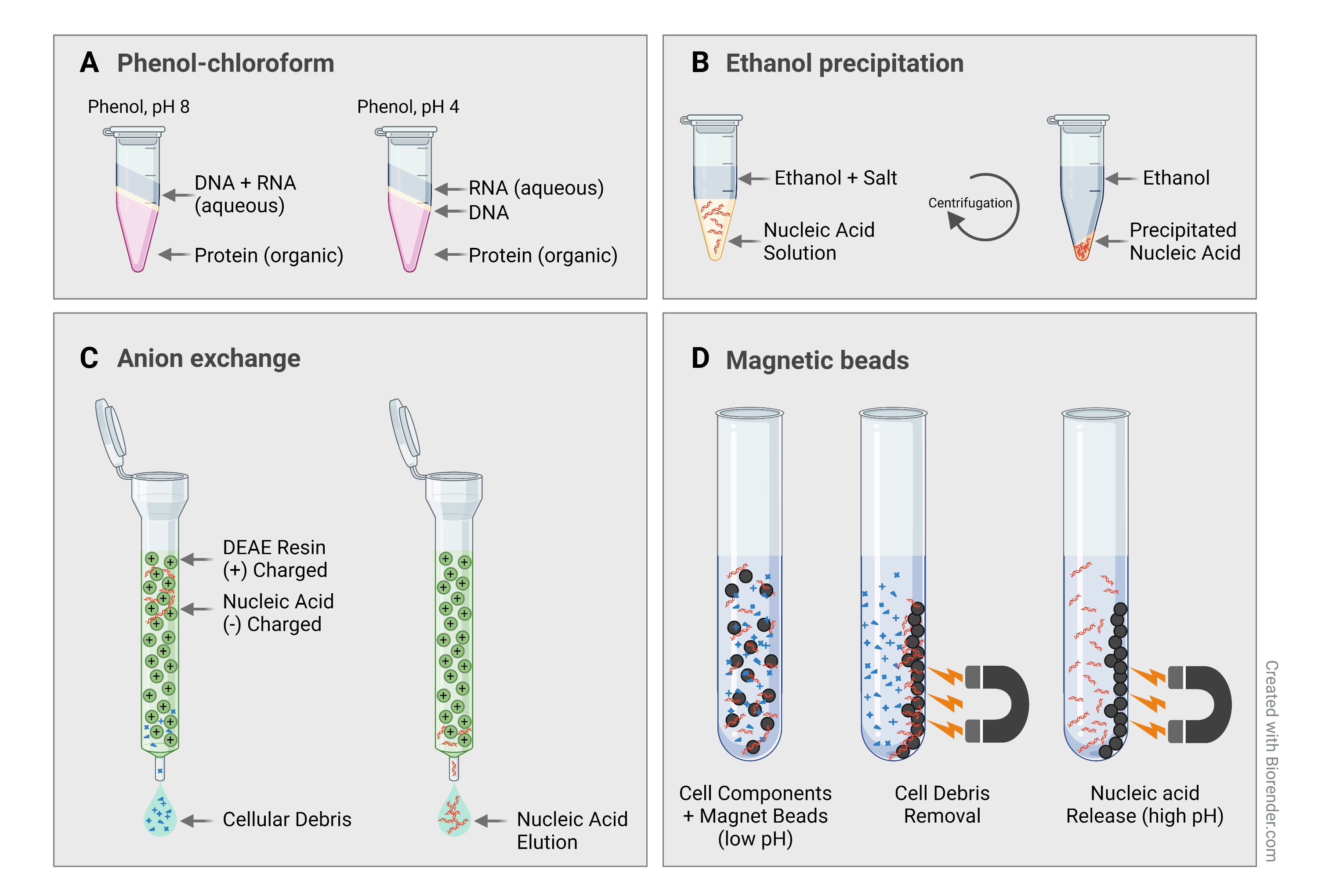
Sample purification
Torres Benito (2022) has a good explanation of sample purification.
- Organic extraction and purification
- Solvents like phenol and chloroform are used to separate proteins and lipids
- DNA/RNA is precipitated from the solution using alcohol
- Silica-based columns
- Spin the sample through a silica matrix
- High-salt buffer causes DNA/RNA to bind to the silica
- Impurities are washed away
- DNA/RNA is eluted using low-salt buffer or water
- Magnetic bead-based purification
- Customizable magnetic beads prepared to stick to desired DNA/RNA
- Magnet is used to hold beads in place for washing stage
- DNA/RNA is washed from beads and eluted
Library preparation
- DNA/RNA is fragmented
- Manually using sonic shearing (e.g. Covaris)
- Enzymatically (e.g. using Qiagen endonuclease digestion kits or Nextera XT DNA library preparation kits).
- Adaptor sequences are attached to the ends of these fragments, serving as binding sites for primers and for anchoring the DNA to a solid support.

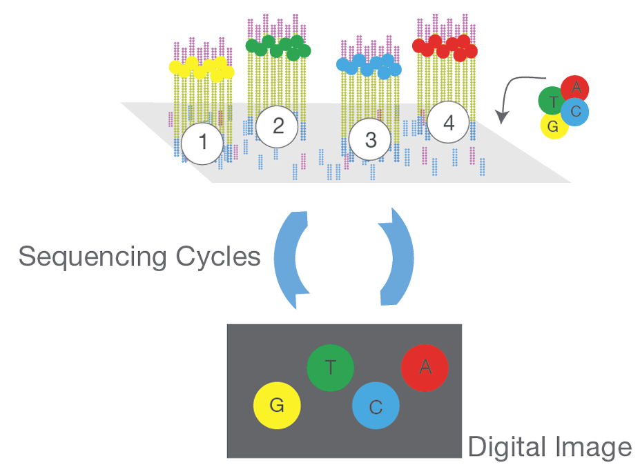
Illumina (Massive Parallel, Short-Read Sequencing)
Illumina sequencing is the most frequently used platform today
Sequencing
- Fragments are attached to the flow cell surface.
- Clusters of identical DNA templates (called “spots” or “clusters”) are formed on the flow cell.
- Fluorescently labeled nucleotides (A, T, C, G) are added in cycles, along with DNA polymerase.
- For each cycle, only one nucleotide can be incorporated, after which a wash step and imaging of the flow cell occur.
- Emitted fluorescence from each cluster identifies the incorporated base.
- Repeat to build the complementary strand.
Read Characteristics
- Produces short reads, typically 50-250 bp
- Paired-end reads are produced when the ends of a longer sequence are sequenced
- High accuracy, reported at 99.9%
Applications
- Small whole genome sequencing (DNA)
- Transcriptomics (RNA)
- 16S metagenomics
- DNA-protein interaction analysis (ChIP-Seq)
- Multiplexing of samples using barcodes
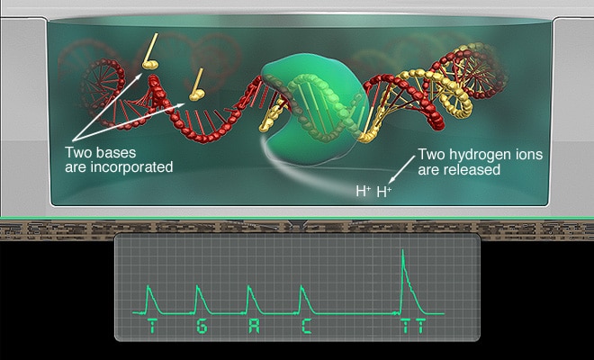
Ion Torrent (Thermo Fisher Scientific)
- Benchtop sequencer released in 2010
- Generates millions of short DNA or RNA reads, similar to Illumina data
- Its size, speed and ease of use make it ideal1 for
- Clinical research - personalized medicine like cancer research
- Microbiology and infectious disease - especially real-time pathogen typing and outbreak surveillance
- Forensic DNA analysis
- Agrigenomics

Sequencing by synthesis
Unlike Illumina’s optical detection, Ion Torrent uses ion semiconductor sequencing technology
It detects hydrogen ions (H+) released during DNA polymerization
Each microwell on the chip contains a single template DNA
Unmodified deoxynucleotide triphosphates (dNTPs) are washed into the microwells, one species at a time (e.g., all A’s, then all T’s).
When a nucleotide is incorporated into a complementary strand, a covalent bond is formed, releasing a phosphate and a hydrogen ion, which is detected by the sensor.
Real-Time, Single Molecule Sequencing (Long-Read Technologies)
- These technologies overcome some limitations of short-read methods by directly sequencing native DNA without prior fragmentation and amplification steps, which can introduce errors and bias
- Long-read technologies yield significantly longer read lengths and provide real-time sequence information
Pacific Biosciences (PacBio)
- PacBio RS system was released in 2011
- Produces long reads, averaging >15 Kb, with some exceeding 100 Kb
Single molecule, real-time (SMRT) sequencing
- A single DNA polymerase is immobilized at the bottom of a nanoscopic microwell called a zero-mode waveguide (ZMW)
- A single DNA template is bound to the polymerase
- Four fluorescently labeled nucleotides are introduced
- As a labeled nucleotide is incorporated a fluorescent a light pulse is produced

Read Characteristics
- Advantages: Long reads are valuable for
- Closing small genomes
- Spanning long, repetitive regions
- Can also be used to determine the methylome (epigenetics) of microorganisms
- Drawbacks:
- Higher sequencing costs
- Higher error rates (especially insertion and deletion errors) compared to Illumina
Oxford Nanopore Technologies (ONT)
- The MinIon device was released in 2014
- Known for its portability

Nanopore sequencing
- A single-stranded DNA molecule is driven by an applied voltage (e.g., 180 mV)
- Passes through a nanopore
- As DNA threads through the nanopore, it
- Causes distinct changes in the ionic current
- Characteristic of the specific nucleotide bases occupying the pore at any given moment

Read characteristics
- Produces variable and very long reads, comparable to PacBio, sometimes up to 900 Kb
- MinIon devices have 512 nanopores, each sequencing approximately 70 bp/second.
- Advantages:
- Extreme portability (USB sequencer)
- Real-time data availability
- Sequencing can be cheaper than PacBio.
- Drawbacks:
- Initially had a high error probability, though recent flow cells (e.g., R10.4.1) report raw read accuracy >99%
- Requires high-quality DNA input and efficient command-line data analysis
Raw Data Generation and Quality Assessment
- Sequence Reads
- Millions of short or long reads
- Represent fragments of the original DNA/RNA
- Data format, typically FASTQ
- Raw sequence reads
- Stores both the nucleotide sequence and its corresponding quality scores for each base
- Quality scores, typically Phred Score (Q)
- Logarithmic measure that reflects the likelihood that a base call is incorrect
- Formula:
Q = -10 log10(p), where ‘p’ is the probability of an incorrect base call- Phred score of 10 (Q10) means 1 error in 10 base calls (90% accuracy)
- Phred score of 20 (Q20) means 1 error in 100 base calls (99% accuracy)
- Phred score of 33 is generally considered a desirable minimum threshold for high-quality data (99.95% accuracy)
- Higher Phred scores indicate greater confidence in the reported base
Initial quality control (QC)
- Assessing the quality of raw data is a critical first step
- Tools like
FastQCare used to generate QC reports, checking for- Consistency
- Base call quality
- Overall data characteristics like GC-content distribution
NGS Data Analysis
- Bioinformatics helps us
- Extracting biological meaning
- Discover relationships between molecular mechanisms and phenotypic behavior
- General workflow
- Preprocessing and QC
- Assembly
- Annotation
- Quantification
- Downstream interpretation
Data preprocessing
- Quality control (QC) using tools like
FastQC- Evaluate the raw sequencing data to ensure it meets acceptable quality thresholds
- Demultiplexing
- DNA barcodes can be added to multiple samples to distinguish different samples
- Barcoded samples can be pooled and sequenced together to save on costs
- Trimming using tools like
trimmomaticto remove- Low-quality bases from the ends of reads
- Adapter sequences
- Barcodes
- Filtering removes reads that are
- Too short
- Contain too many ambiguous bases
- Contain potential sequencing errors (e.g. remove low-frequency k-mers to correct errors)
- Denoising
- Computational methods to correct errors introduced during the sequencing process
- Denoising algorithms use statistical models that consider quality scores to estimate the probability of sequence errors
Denoising is especially important in 16s RNA amplicon sequencing to distinguish:
- Low-frequency variants (real) from PCR amplified sequencing errors (not real)
- Number of truly unique sequences, used as a proxy for the number of species / OTUs
- Closely related species with highly similar amplicon sequences
- Quality control
- Processed reads are re-evaluated to evaluate the efficacy of the preceding steps
- Normalization of expression and abundance
- Essential for ensuring comparability across different datasets and samples
- Important for
- RNA expression
- Metabolomics
- Proteomics
Sequence assembly
Goal: Reconstruct longer, contiguous DNA sequences (contigs, scaffolds, or even full chromosomes) from many sequence reads.

- De novo assembly
- Used when no reference genome is available
- Used to detect structural variation (e.g. large indels, chromosomal inversions / duplications)
SPAdesis a popular tool for genomes and single-cell sequencing
- Reference-guided assembly/mapping
- Aligning reads to an existing, closely related reference genome
Bowtieis used for aligning sequence reads in RNA-seqHisat2is used for spliced read mappingSamtoolshandles mapped reads
- Assembly quality assessment
- N50: length of the shortest contig such that 50% of the assembly is covered by contigs of this length or longer
- NG50: N50 but with reference to the known genome size
- Completeness:
- How many genes are represented when mapping RNA-seq data?
- For de novo assembly, Benchmarking Universal Single-Copy Orthologs (BUSCO) is a set of core genes that are highly conserved and expected to be present across a specific taxonomic lineage
Annotation
Goal: Identify and label all relevant biological features within the assembled genomic sequence.
Prediction of coding genes
Identification of other structural genes (e.g. rRNA genes)
- Functional prediction
- Existing protein databases can be used to infer function based on similarity (e.g. NCBI’s GenPept, UniProt)
- Functional annotation (e.g. using Gene Ontology (GO) terms)
- Common tools:
- RAST (Rapid Annotation using Subsystems Technology) for microbial genomes
- BlastKOALA for single genomes
- GhostKOALA for metagenomes
- Prokka for prokaryotic genome annotation
- Prodigal for prokaryotic gene recognition
- Challenges: Automated annotation methods can be faster but may reduce confidence due to dissimilar results from different servers/databases, and often require manual curation for accuracy.
Quantification and differential expression analysis
Goal: Measure the gene expression or protein abundance and identify changes between different experimental conditions.
- Transcriptomics (RNA-seq)
- Measures the level of transcribed genes to detect active genes genome-wide
- Quantification
- After alignment of reads to a reference genome, number of reads mapping to each gene or transcript is quantified
- Differential gene expression (DGE): Statistical analysis to identify genes whose expression levels significantly change between conditions (e.g., treated vs. control samples)
- Tools:
DESeq2EdgeRBaySeqDRIMSeqSleuthStringTie
Downstream Analysis and Interpretation
Statistical analysis and visualization
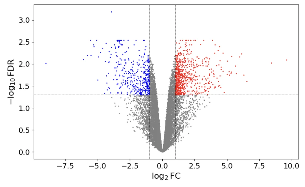
Volcano plots visualize differential expression / abundance in context with statistical significance. Arshad (2024) gives step-by-step instructions for creating volcano plots in R.
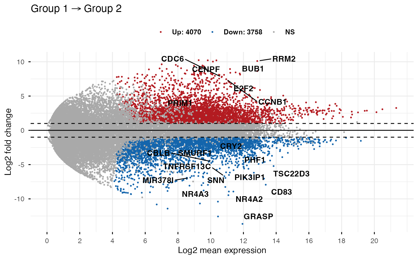
MA-plots visualize protein differential abundance. Red points represent genes that are upregulated in Group 1 compared to Group 2, and blue points represent downregulation (Kassambara 2016).
ggpubr package.Principal Component Analysis (PCA) can be used for dimensionality reduction and visualizing data clustering (Cheng (2022) has a nice discussion of PCA).

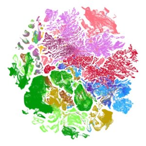
Uniform manifold approximation and projection (UMAP) is a more appropriate dimensionality reduction technique for data that violate the linearity assumption of PCA. Mueler and Casimo (2025) have a good description of UMAP with examples.
Enrichment or pathway analysis can identify biological pathways or gene sets that are statistically over-represented in a list of differentially expressed genes or proteins. For example the following are widely used:
- KEGG (Kyoto Encyclopedia of Genes and Genomes)
- Reactome
Quantitative protein data can be used to reconstruct protein interactions and signaling networks. The STRING database provides quality-controlled protein-protein association networks.
Machine learning applications
Increasingly used to glean insights from complex biological data.
- Sample Clustering
- Classification
- Deep Learning (e.g. AlphaFold for protein structure prediction)
Challenges in NGS Data Science
Data volume and storage
Computational resources
Data quality issues
- Sparsity (e.g. in scRNA-seq, a large fraction of observed zeros (dropout events) can hinder downstream analysis)
- Missing values (e.g. low-abundance proteins can result in missing values)
- Noise and errors (e.g. Technical variability)
Model interpretability, especially in deep learning
Data integration