20 NGS Assembly Practice

Author

Affiliation

Dr Randy Johnson

Hood College

Published

September 10, 2025

Introduction

Today we will pick up where we left off last week and perform the following steps:

Trim Illumina adapters from our reads

Start by uploading the paired end reads for the file we were exploring last week. You can fetch the fastq file here. You should now have the following fastq files available on Galaxy:

SRR2584863_1.trim.sub.fastq
SRR2584863_2.trim.sub.fastq

Trimming

Open the Trimmomatic tool on Galaxy.

Select the following inputs and parameters for Trimmomatic:
- Singe-end or paired-end reads: paired-end
  - Input FASTQ file 1: SRR2584863_1.trim.sub.fastq
  - Input FASTQ file 2: SRR2584863_2.trim.sub.fastq
- Perform Illuminaclip step: Yes
  - Standard adapter sequences
  - Adapter sequences: Nextera (paired-end)
  - Keep all other defaults
- Trimmomatic operation:
  - Sliding window trimming
  - Number of bases to average across: 4
  - Average quality required: 20
- Trimmomatic operation (insert a second operation):
  - MINLEN: 25
- Keep all other defaults
Rerun FastQC to verify that the trim step was successful.
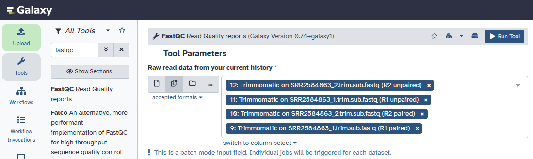
- We now have 4 files to run. Select the multiple datasets option for the input field and select the output files from Trimmomatic.

QC

The unpaired read files are going to be very small and hard to tell what is going on with any reliability, but the two paired files still don’t look quite right.

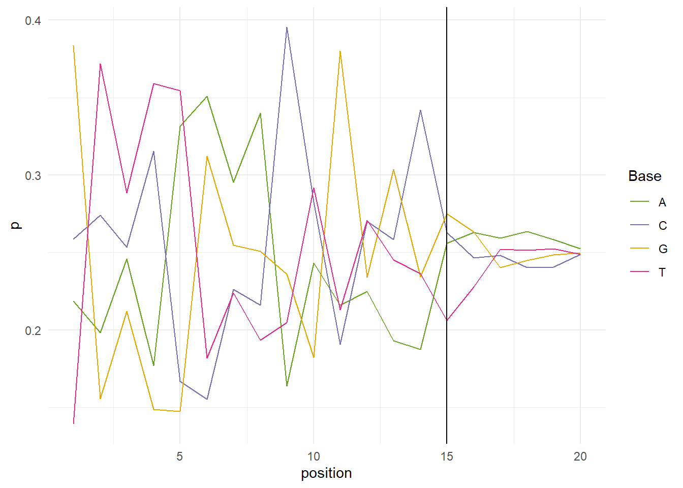
A warning is thrown by FastQC if the difference between two bases is greater than 10%, and an error is thrown if the difference is greater than 20%. If we look at the per sequence content plot of the first 20 positions of SRR254863_1, it looks like we should be find trimming the head of our sequences up to 15 base pairs.

Code

library(ShortRead) # install with BiocManager::install("ShortRead")
library(stringr)
library(tidyr)
library(ggplot2)
library(RColorBrewer)

root <- here::here()

# read sequences
reads <- readFastq(file.path(root, 'data', 'ngs', 'SRR2584863_1.trim.sub.fastq')) |>
  sread()

# split out nucleotides in the first 20 positions
nbp <- 20
bp_by_pos <- subseq(reads, start = 1, end = nbp) |>
  as.character() |>
  str_split('') |>
  unlist() |>
  matrix(ncol = nbp, byrow = TRUE)

# set up our own per base sequence content plot
pb <- tibble(position = 1:nbp,
             A  = apply(bp_by_pos == 'A', 2, mean),
             C  = apply(bp_by_pos == 'C', 2, mean),
            `T` = apply(bp_by_pos == 'T', 2, mean),
             G  = apply(bp_by_pos == 'G', 2, mean)) |>
  pivot_longer(cols = 2:5, names_to = 'Base', values_to = 'p')

ggplot(pb, aes(position, p, color = Base)) +
  geom_line() +
  theme_minimal() +
  geom_vline(xintercept = 15) +
  scale_color_manual(values = brewer.pal(n = 7, name = 'Dark2')[c(5,3,6,4)])

Per base sequence content over the first 20 positions of SRR2584863_1

Run Trimmomatic again using the settings as above plus an additional Trimmomatic operation:
- HEADCROP: 15
Rerun FastQC on the 2 pared files created by Trimmomatic (we’ll skip the unpaired files this time).

Read mapping

Once we are happy with our QC report, let’s move on to mapping the reads to a reference genome and calling some variants!

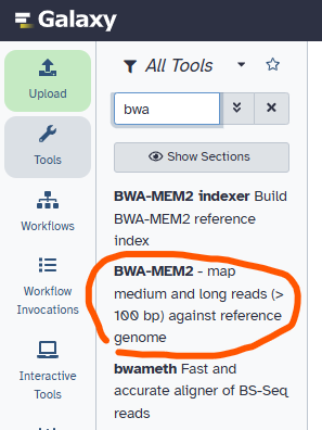
Open the BWA-MEM2 tool in Galaxy and select the following as inputs:
- Built-in genome: Escherichia coli O157:H7 str. Sakai (GCF_000008865.2)
- Paired reads
  - Trimmomatic on SRR2584863_1.trim.sub.fastq (R1 paired)
  - Trimmomatic on SRR2584863_2.trim.sub.fastq (R2 paired)

Variant calling

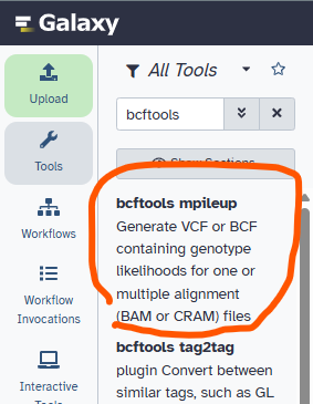
Open the bcftools mpileup tool and select the following inputs:
- Input: xx: BWA-MEM2 on data yy and data zz (mapped reads in BAM format) where xx and yy correspond to the job numbers for the different steps we’ve run thus far.
- Use the same locally cached Ecoli reference genome we used above: Escherichia coli O157:H7 str. Sakai (GCF_000008865.2)

Open the bcftools call tool and select the following inputs:
- VCF/BCF data: xx: bcftools mpileup on data yy where xx and yy correspond to the job ids for the previous two steps.
- Calling method: consensus caller

Annotation

Open the bcftools csq tool and select the following inputs:
- VCF/BCF data: xx: bcftools call on data yy where xx and yy are the job ids for the previous two steps.
- Reference genome: Escherichia coli O157:H7 str. Sakai (GCF_000008865.2)
- GFF3 annoation file: GCF_000008865.2_ASM886v2_genomic.gff.gz (this can also be found on the corresponding NCBI page under FTP)

I had trouble getting this to work, so let’s try a different approach. This will take longer to run, since we aren’t using a pre-annotated gff file.

Convert your bcf file to a fasta file with the bcftools consensus tool. Galaxy should remember your reference genome.

Annotate the consensus sequence with the Bakta tool - use the defaults.

This gives us several outputs (see Ensembl for additional information):

Summary: I think this can be ignored, as it seems to be identical to the gff file. There are some visualization tools you could use to look at the information in the gff file, but these visualizations are rudimentary.
gff: The gff file contains annotations for our sample’s genome. Columns include:
- Contig where the feature was found
- Database where the annotations come from
- Type of annotation, for example: CDS (coding DNA sequence), ncRNA (non-coding RNA), regulatory region
- Start and end positions of the region
- Score: E-value for the feature (if available)
- Strand (+/-)
- Phase: indicates the first base of the reading frame where
  - 0: feature starts on the first base of a codon
  - 1: feature starts on the second base of a codon
  - 2: feature starts on the third base of a codon
- Metadata with additional information regarding the region
A fasta file with all nucleotide sequences for each feature in the gff file
A ciros plot of the data with one section per contig. The location of features is shown in the outer rings and the gc content (red/green) and gc content skew (blue/gold) are shown in the inner rings.