# tidyverse packages for data wrangling
library(dplyr)
library(tidyr)

# graphics packages
library(matrixBP)
library(RColorBrewer)
library(cowplot)
library(ggrepel)
library(ComplexHeatmap)

theme_set(theme_cowplot())25 Metabolomics Figures
Today we will practice generating some of the figures that are typical of metabolomics data analysis. First, you’ll need to load/install a few R packages:
Note
You can install the matrix bar plot package with:
devtools::install_github('IDSS-NIAID/matrixBP')Data
The matrixBP package comes with a simulated lipidomics data set that we will be visualizing today.
data(metlip)# A tibble: 768 × 7
Lipid Group Acyl_1 Acyl_2 sample log2FC neg_log_p
<chr> <fct> <chr> <chr> <chr> <dbl> <dbl>
1 PC(14:0_14:0) PC C14:0 C14:0 A -0.205 1.83
2 PC(14:0_16:0) PC C14:0 C16:0 A -0.237 1.66
3 PC(14:0_18:0) PC C14:0 C18:0 A -0.712 2.45
4 PC(16:1_18:0) PC C16:1 C18:0 A -0.239 2.26
5 PC(18:0_18:0) PC C18:0 C18:0 A 0.434 1.73
6 PC(14:0_18:1) PC C14:0 C18:1 A -0.241 1.92
7 PC(16:1_18:1) PC C16:1 C18:1 A 0.543 2.70
8 PC(18:0_18:1) PC C18:0 C18:1 A -0.264 1.69
9 PC(18:1_18:1) PC C18:1 C18:1 A -0.208 1.60
10 PC(16:0_18:2) PC C16:0 C18:2 A -0.240 2.17
# ℹ 758 more rowsThis simulated data consists of data from an imaginary study in which each individual (A, B, C, D) is sampled before and after treatment. Change in lipid abundance is measured between the two time points.
Each lipid in the data set is categorized by group. Gemini’s summarization of these groups follows.
Gemini on lipid groups
These abbreviations represent major classes of lipids, primarily glycerophospholipids and sphingolipids, which are the structural and signaling components of cell membranes.
Here is a breakdown of the groups, their full names, and their primary roles in biology:
🔬 Glycerophospholipids (Structural & Signaling)
Glycerophospholipids (often called phospholipids) are built on a glycerol backbone with two fatty acid chains and a phosphate group linked to a polar head group. Most of the lipids in your list fall into this category.
| Group | Full Name | Type / Charge at pH 7 | Primary Biological Function |
| PC | Phosphatidylcholine | Zwitterionic (Neutral) | Most abundant membrane lipid in eukaryotes. Essential for cell membrane structure, fluidity, and integrity. |
| PE | Phosphatidylethanolamine | Zwitterionic (Neutral) | Second most abundant. Crucial for membrane fusion and shaping membrane curvature due to its cone shape. Important in mitochondrial function. |
| PI | Phosphatidylinositol | Negative | A key component in cell signaling. Its head group can be phosphorylated to create Phosphoinositides (PIPs), which regulate cell growth, migration, and membrane trafficking. |
| PS | Phosphatidylserine | Negative | Primarily located on the inner leaflet of the plasma membrane. Its exposure on the outer leaflet is a key “eat me” signal for cells undergoing apoptosis (programmed cell death). |
| PG | Phosphatidylglycerol | Negative | Important component of pulmonary surfactant (in the lungs) and is a precursor for Cardiolipin (a critical lipid in the inner mitochondrial membrane). |
🔍 Lysophospholipids (Lyso- Lipids)
The “Lyso_” prefix indicates a lipid that has lost one of its two fatty acid chains (usually at the sn-2 position of the glycerol backbone). This loss is typically catalyzed by phospholipase A2 (PLA2).
| Group | Full Name | Type / Charge at pH 7 | Primary Biological Function |
| Lyso_PC | Lysophosphatidylcholine | Zwitterionic (Neutral) | Potent signaling molecule involved in inflammation and the immune system. Can be a precursor for other bioactive lipids. |
| Lyso_PE | Lysophosphatidylethanolamine | Zwitterionic (Neutral) | Involved in cell differentiation, migration, and acts as a signaling molecule. Also acts as a precursor for PE synthesis. |
| Lyso_PI | Lysophosphatidylinositol | Negative | Less studied than Lyso_PC, but also recognized as a potential signaling lipid and a potential marker in inflammation or cancer. |
| Lyso_PG | Lysophosphatidylglycerol | Negative | A breakdown product of PG; may be involved in membrane dynamics and remodeling. |
🧬 Sphingolipids & Other Classes
Sphingo
Refers to: Sphingolipids, a class built on a sphingoid base (like sphingosine) rather than glycerol.
Key Example Subclass: Sphingomyelin (SM), which is structurally similar to PC (sharing the choline head group) but uses a ceramide backbone.
Function: Sphingolipids are crucial for cell recognition, adhesion, and signaling. They are heavily involved in forming rigid membrane domains called lipid rafts, which are important for signal transduction.
Neutral
Refers to: Neutral Lipids (or neutral glycerolipids).
Key Example Subclasses: This group typically includes Triacylglycerols (TAGs or Triglycerides) and Diacylglycerols (DAGs).
Function:
TAGs: Primarily serve as energy storage (fat) in cells.
DAGs: Important second messengers in cell signaling pathways (e.g., activating Protein Kinase C).
Matrix Bar Plot
We can view patterns by lipid group, across samples with a matrix bar plot of the data:
# define colors for each lipid group
grp_colors <- levels(metlip$Group) |>
  length() |>
  brewer.pal('Set3')
names(grp_colors) <- levels(metlip$Group)

# matrix bar plot
matrix_barplot(metlip, aes(x = Lipid, y = neg_log_p, color = log2FC),
               cols = vars(Group), rows = vars(sample), facet_colors = grp_colors) |>
  mBP_legend()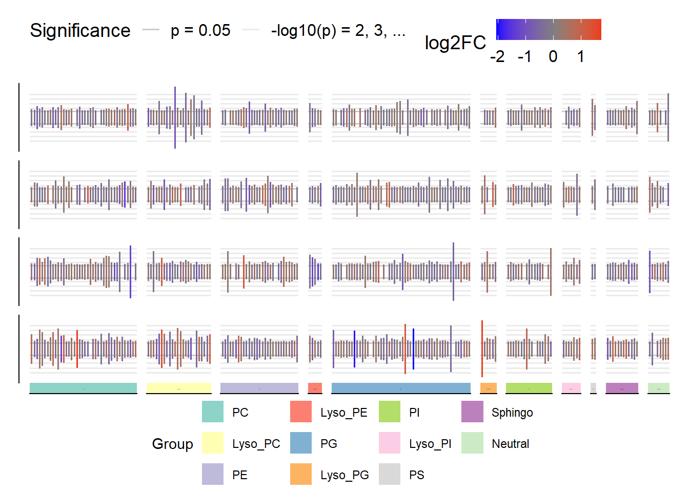
Volcano Plot
Since we don’t have individual abundances for before and after treatment, we can’t calculate mean abundance for an MD-plot. We will create a volcano plot instead.
# Add a column to the data frame to indicate significance
metlip_volcano <- mutate(metlip,
                         significant = neg_log_p > 1.3 & abs(log2FC) > 1)

# Create the volcano plot
ggplot(metlip_volcano, aes(x = log2FC, y = neg_log_p, color = significant)) +
  geom_point() +
  scale_color_manual(values = c("black", "red")) +
  labs(title = "Volcano Plot",
       x = "log2 Fold Change",
       y = "-log10(p-value)") +

  geom_text_repel(data = subset(metlip_volcano, significant),
                  aes(label = Lipid),
                  size = 3,
                  box.padding = unit(0.5, "lines"),
                  point.padding = unit(0.5, "lines"))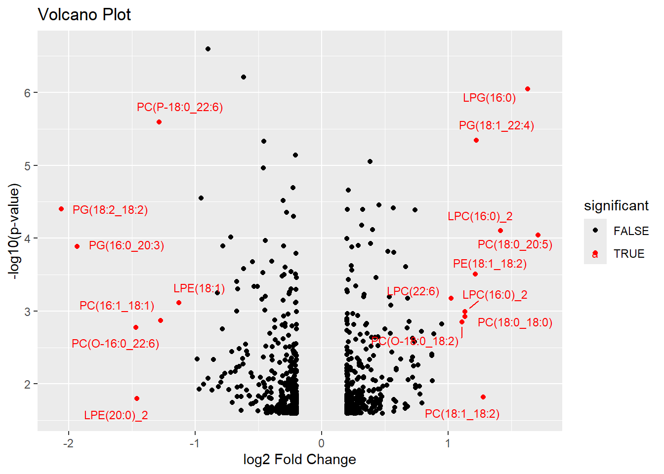
PCA Plot
Lastly we’ll create a PCA plot of the data. We don’t have the abundances for before and after treatment for each sample, so instead we’ll look at the relationships between samples. This is less interesting for these data, but it will give us practice with PCA.
# Prepare the data for PCA
pca_data <- metlip |>
  select(sample, Lipid, log2FC) |>
  pivot_wider(names_from = Lipid, values_from = log2FC) |>
  as.data.frame()

rownames(pca_data) <- pca_data$sample
pca_data <- pca_data[,-1]

# fill in missing values with column means
col_means <- colMeans(pca_data, na.rm = TRUE)
for(j in 1:ncol(pca_data))
  pca_data[is.na(pca_data[,j]),j] <- col_means[j]

# Perform PCA
pca_res <- prcomp(pca_data, scale. = TRUE)

# Create a data frame for plotting
pca_plot_data <- data.frame(
  sample = rownames(pca_data),
  PC1 = pca_res$x[,1],
  PC2 = pca_res$x[,2]
)

# Create the PCA plot
ggplot(pca_plot_data, aes(x = PC1, y = PC2, color = sample)) +
  geom_point(size = 3) +
  labs(title = "PCA of Metabolomics Data",
       x = paste0("PC1 (", round(summary(pca_res)$importance[2,1]*100, 1), "%)"),
       y = paste0("PC2 (", round(summary(pca_res)$importance[2,2]*100, 1), "%)")) +
  theme_cowplot()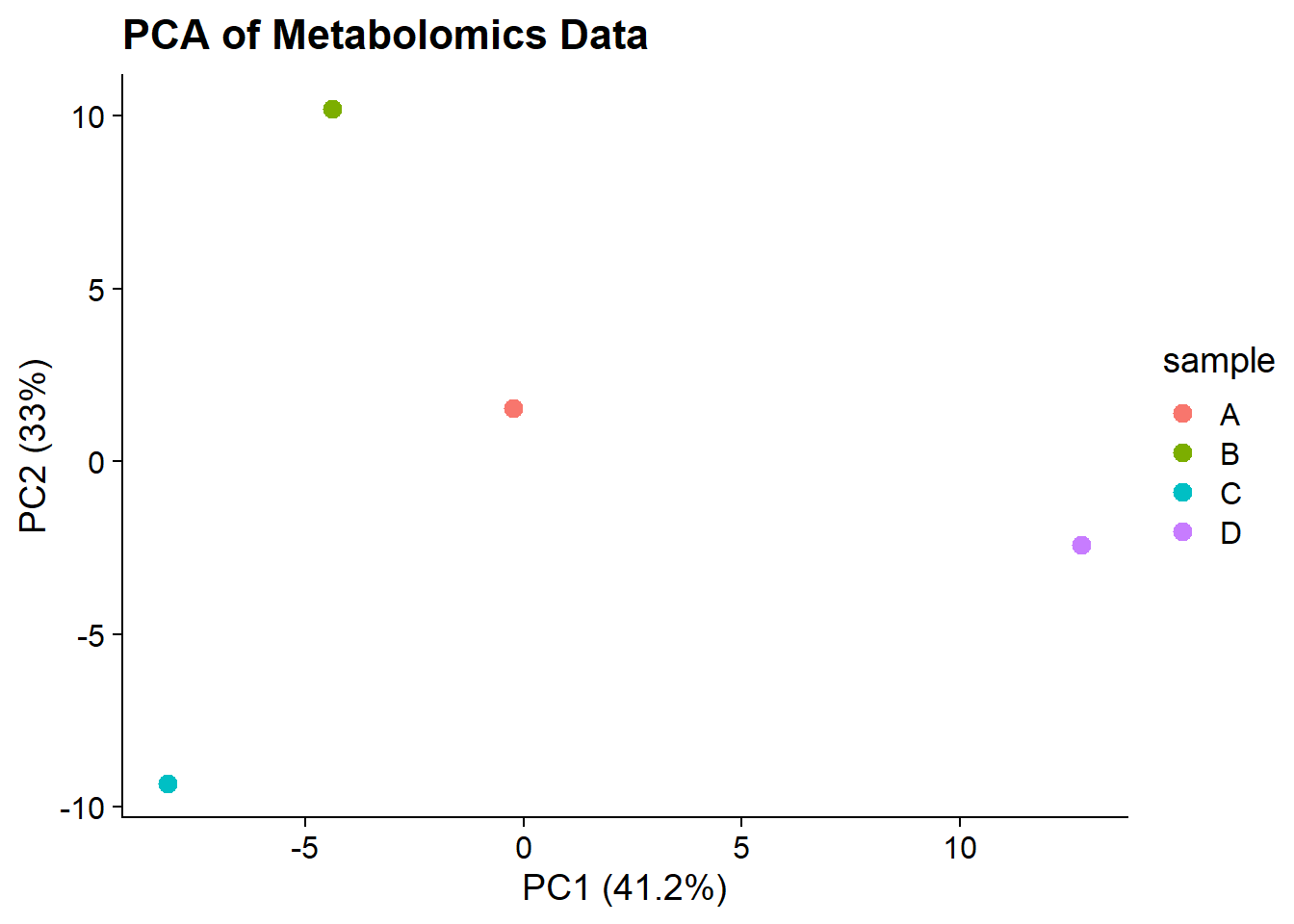
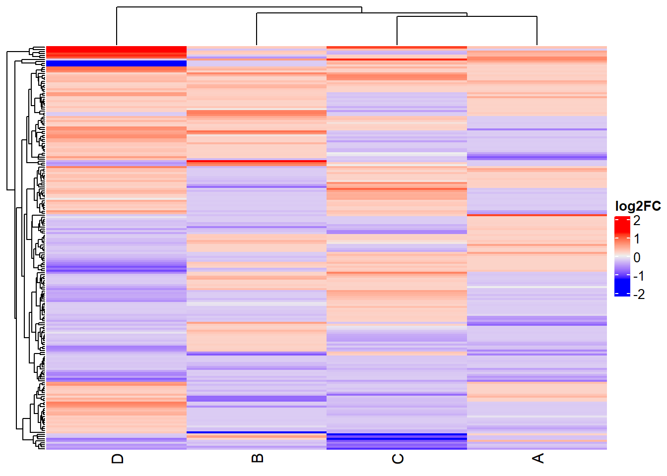
Heatmap
# Prepare the data for the heatmap
heatmap_data <- t(pca_data)

# Create the heatmap
Heatmap(heatmap_data,
        name = "log2FC",
        cluster_rows = TRUE,
        cluster_columns = TRUE,
        show_row_names = FALSE)