# data analysis follows tutorial at# https://bioconductor.org/packages/release/bioc/vignettes/DEP/inst/doc/DEP.htmllibrary(DEP)library(dplyr)# The data is provided with the packagedata <- UbiLength# We filter for contaminant proteins and decoy database hits, which are indicated by "+" in the columns "Potential.contaminants" and "Reverse", respectively. data <-filter(data, Reverse !="+", Potential.contaminant !="+")# Are there any duplicated gene names?data$Gene.names %>%duplicated() %>%any()
[1] TRUE
# Make a table of duplicated gene namesdata %>%group_by(Gene.names) %>%summarize(frequency =n()) %>%arrange(desc(frequency)) %>%filter(frequency >1)
# Make unique names using the annotation in the "Gene.names" column as primary names and the annotation in "Protein.IDs" as name for those that do not have an gene name.data_unique <-make_unique(data, "Gene.names", "Protein.IDs", delim =";")# Are there any duplicated names?data$name %>%duplicated() %>%any()
[1] FALSE
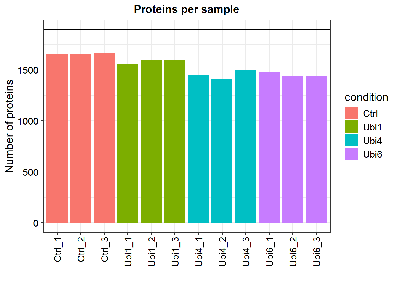
# Generate a SummarizedExperiment object using an experimental designLFQ_columns <-grep("LFQ.", colnames(data_unique)) # get LFQ column numbersexperimental_design <- UbiLength_ExpDesigndata_se <-make_se(data_unique, LFQ_columns, experimental_design)# Generate a SummarizedExperiment object by parsing condition information from the column namesLFQ_columns <-grep("LFQ.", colnames(data_unique)) # get LFQ column numbersdata_se_parsed <-make_se_parse(data_unique, LFQ_columns)# Filter for proteins that are identified in all replicates of at least one conditiondata_filt <-filter_missval(data_se, thr =0)# Less stringent filtering:# Filter for proteins that are identified in 2 out of 3 replicates of at least one conditiondata_filt2 <-filter_missval(data_se, thr =1)plot_numbers(data_filt)
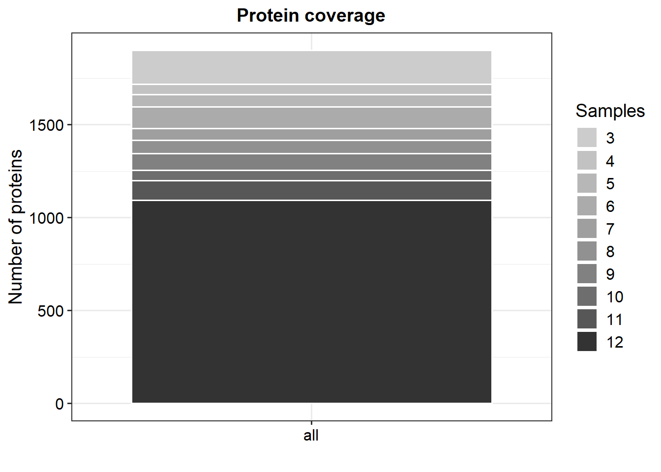
plot_coverage(data_filt)
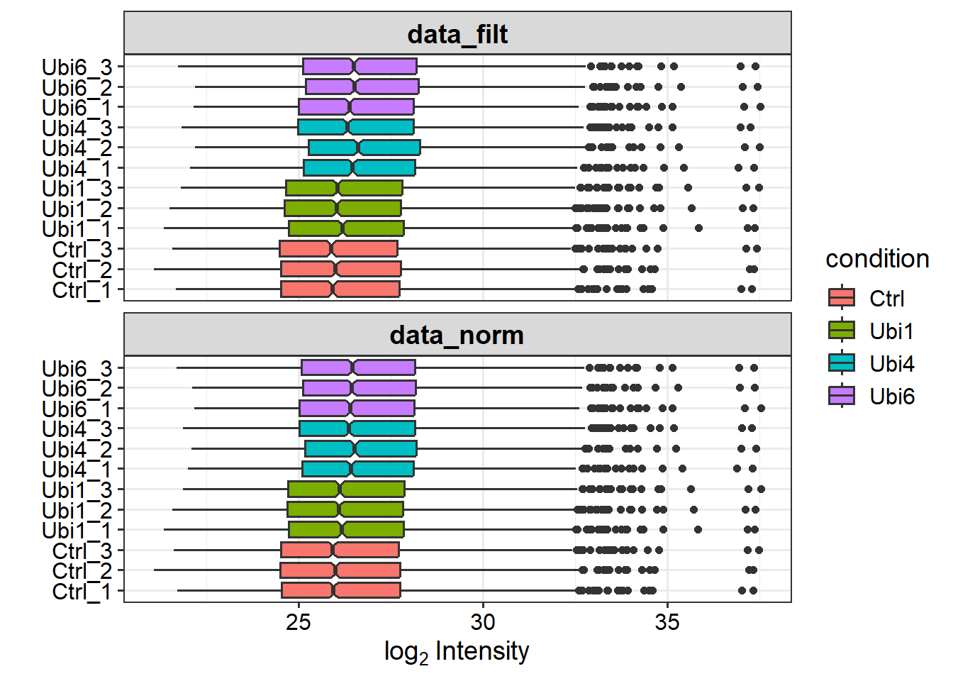
# Normalize the datadata_norm <-normalize_vsn(data_filt)# Visualize normalization by boxplots for all samples before and after normalizationplot_normalization(data_filt, data_norm)
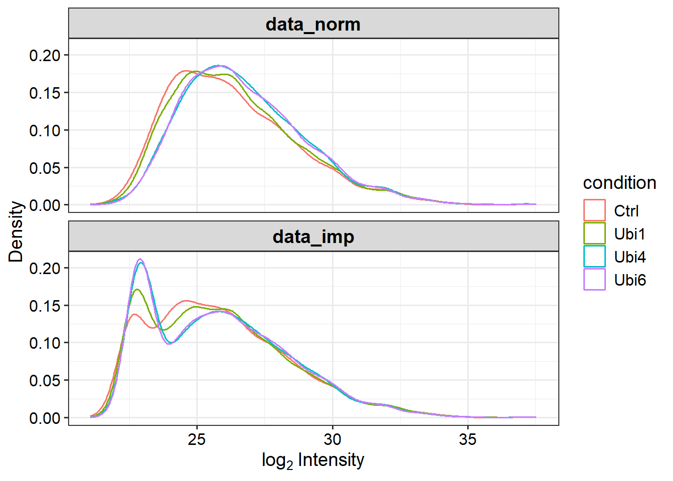
# Impute missing data using random draws from a Gaussian distribution centered around a minimal value (for MNAR)data_imp <-impute(data_norm, fun ="MinProb", q =0.01)
[1] 0.2608395
# Plot intensity distributions before and after imputationplot_imputation(data_norm, data_imp)
Differential enrichment analysis based on linear models and empherical Bayes statistics
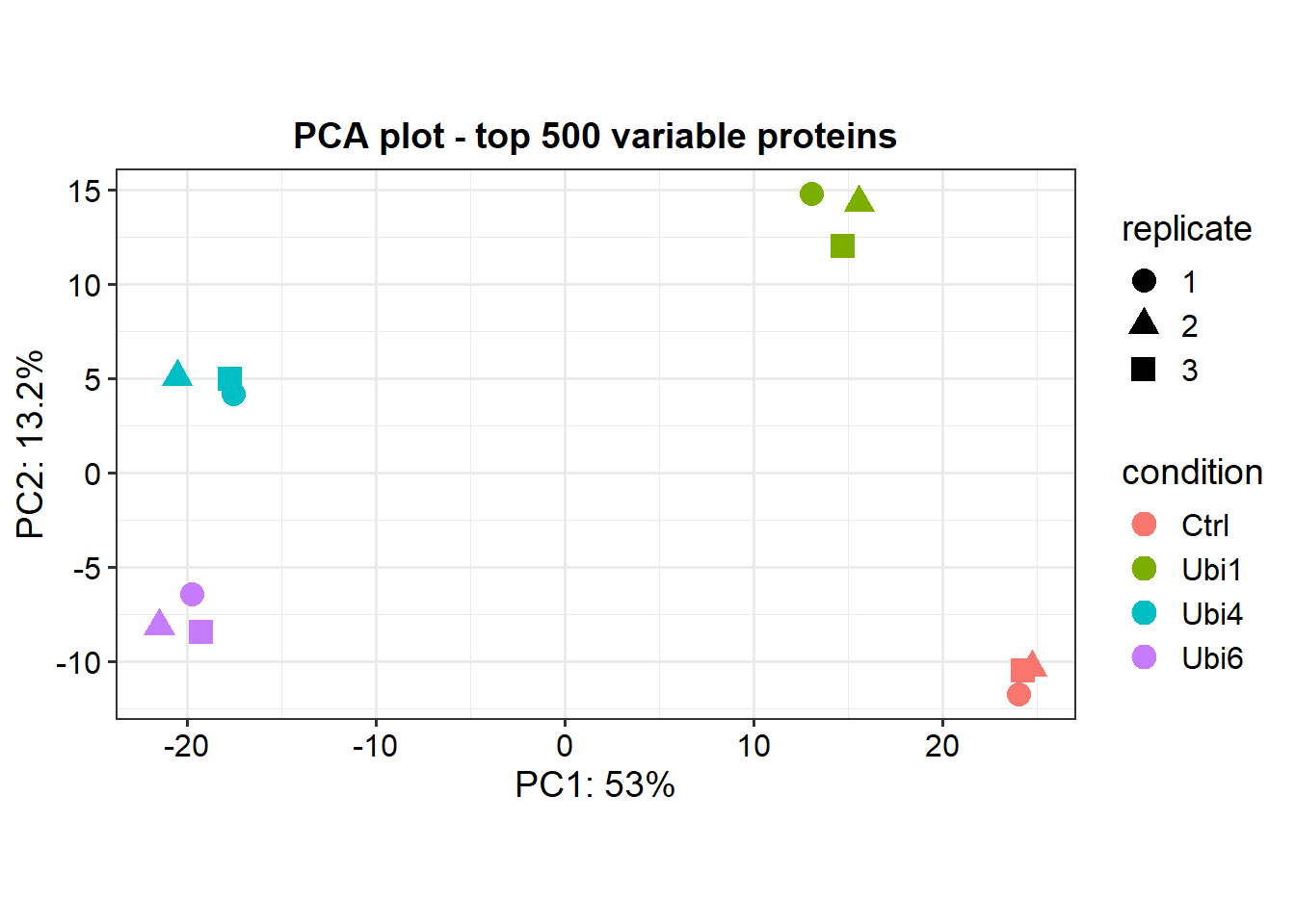
# Test every sample versus controldata_diff <-test_diff(data_imp, type ="control", control ="Ctrl")# Test all possible comparisons of samplesdata_diff_all_contrasts <-test_diff(data_imp, type ="all")# Test manually defined comparisonsdata_diff_manual <-test_diff(data_imp, type ="manual", test =c("Ubi4_vs_Ctrl", "Ubi6_vs_Ctrl"))# Denote significant proteins based on user defined cutoffsdep <-add_rejections(data_diff, alpha =0.05, lfc =log2(1.5))# Plot the first and second principal componentsplot_pca(dep, x =1, y =2, n =500, point_size =4)
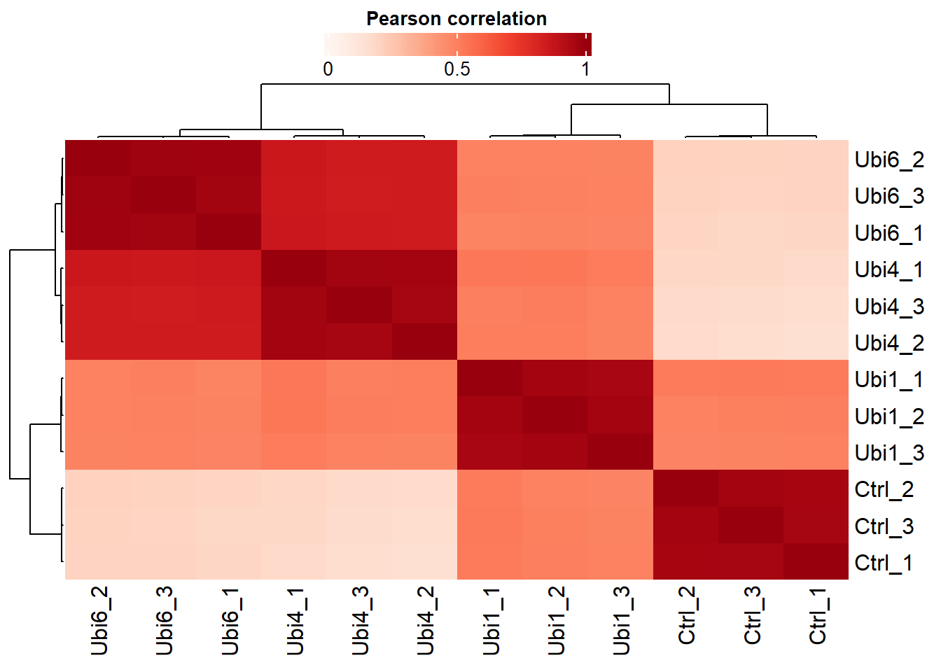
# Plot the Pearson correlation matrixplot_cor(dep, significant =TRUE, lower =0, upper =1, pal ="Reds")
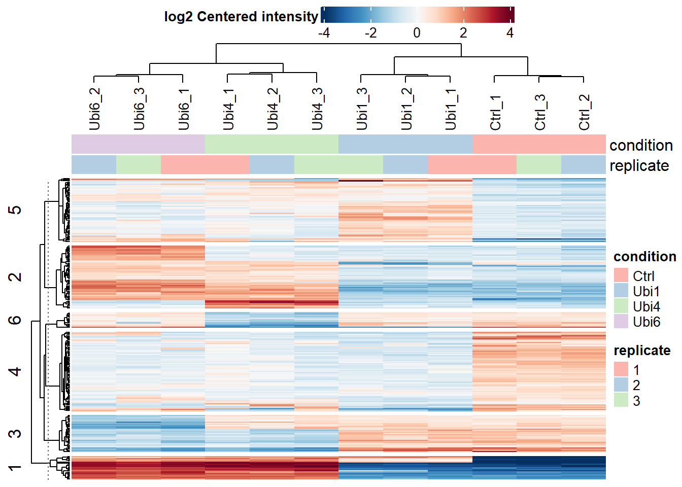
# Plot a heatmap of all significant proteins with the data centered per proteinplot_heatmap(dep, type ="centered", kmeans =TRUE, k =6, col_limit =4, show_row_names =FALSE,indicate =c("condition", "replicate"))
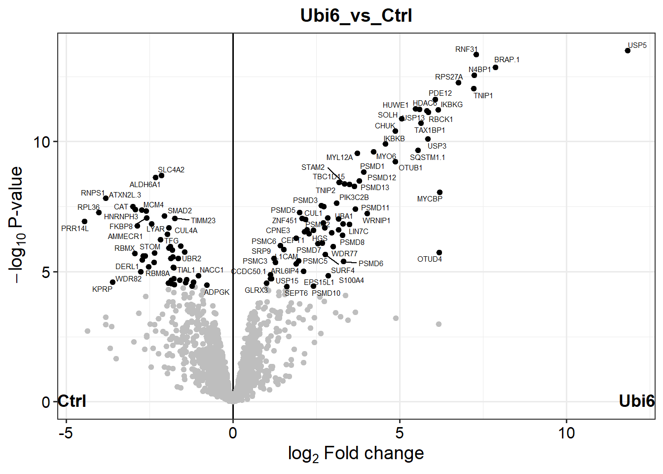
# Plot a volcano plot for the contrast "Ubi6 vs Ctrl""plot_volcano(dep, contrast ="Ubi6_vs_Ctrl", label_size =2, add_names =TRUE)
Make your own volcano plot
# save resultsget_results(dep) |>write.csv(file ='data/prot/UbiLength.csv')
Download the results from our differential enrichment analysis here.
Cox, Jürgen, and Matthias Mann. 2008. “MaxQuant Enables High Peptide Identification Rates, Individualized p.p.b.-Range Mass Accuracies and Proteome-Wide Protein Quantification.”Nature Biotechnology 26 (12): 1367–72. https://doi.org/10.1038/nbt.1511.
Zhang, Xiaofei, Arne H Smits, Gabrielle Ba Van Tilburg, Huib Ovaa, Wolfgang Huber, and Michiel Vermeulen. 2018. “Proteome-Wide Identification of Ubiquitin Interactions Using UbIA-MS.”Nature Protocols 13 (3): 530–50. https://doi.org/10.1038/nprot.2017.147.